Custom Losses at Scale with River Symbolic Engine

Research in LLM post-training keeps introducing new objectives, auxiliary losses, and weighting schemes.
River provides a way to experiment with these ideas beyond a fixed menu of built-in losses.

Today, we're bringing custom loss computation directly to the training backend, powered by the River Symbolic Engine. Simply write your custom loss in PyTorch, and River automatically compiles and executes it across GPUs, handling memory management and backpropagation for you.

Most post-training APIs require clients to compute custom losses locally. This introduces unnecessary communication, redundant computation, and significant client-side complexity. Tinker reports up to 1.5× the FLOPs and 3× the wall-clock time of a standard forward-backward pass^[1], while also requiring the client to perform complex loss and gradient computation.

Instead, River captures supported tensor operations as a symbolic graph that can be validated and optimized on the backend. The loss and its backward pass run beside the model's logits, within a single forward-backward call. This keeps loss computation on the training workers and avoids the extra full-model forward pass and client-side gradient exchange.

Example: Decision Models

Decision models act as general-purpose classifiers, returning a probability for each label given an input and a set of choices. For example, they can determine whether an agent's next action requires approval, whether a comment violates community rules, or which move to make in a game. Models such as Jev^[2] demonstrate the potential of this approach. We can fine-tune an LLM for these tasks by representing each choice with one token and training cross-entropy over just those candidates. Each sequence in this example contains one decision position:

import torch.nn.functional as F
from river_client import CustomLoss

def decision_loss(logits, inputs):
    log_probs = F.log_softmax(logits, dim=-1)
    candidate_log_probs = log_probs.gather(-1, inputs["candidates"]).float()
    log_normalizer = (candidate_log_probs + inputs["log_mask"]).logsumexp((0, 1))
    target_log_prob = (inputs["target"] * candidate_log_probs).sum()
    return (log_normalizer - target_log_prob) * inputs["weight"].sum()

K = ...  # Number of choices, each mapped to a distinct token in the prompt.
schema = {
    "candidates": {"dtype": "int64", "shape": ("T", K)},  # Valid token IDs at every position.
    "target": {"dtype": "float32", "shape": ("T", K)},  # One-hot at the decision position; zero elsewhere.
    "log_mask": {"dtype": "float32", "shape": ("T", 1)},  # 0 at the decision position; -1e30 elsewhere.
    "weight": "float32",  # Zero outside the decision position; include class and batch scaling.
}
loss = model.prepare_loss(CustomLoss(decision_loss, inputs=schema))

This keeps the model's existing output head, allowing a single forward pass to score all choices at the decision position. Fine-tuning with this objective then adapts its language or visual understanding to the application's decisions.

From user-defined loss to parallel execution

River captures your objective's supported tensor operations as a typed symbolic graph. The capture process runs locally on the client and needs no GPU. River then validates the graph and turns it into a program for its training workers. The loss and its backward pass run entirely on River's backend, beside the model's logits.

A custom loss receives logits of shape [T, V] and declared input columns for one example: T token positions and a vocabulary of size V. It returns a scalar loss. Here is a weighted cross-entropy objective and the graph captured from it:

import torch
def weighted_cross_entropy(logits, data):
    logp = logits.log_softmax(
        -1, dtype=torch.float32)
    selected = logp.gather(
        -1, data["target_ids"])
    per_token = selected.sum(-1)
    return -(
        per_token * data["weights"]
    ).sum()

def rows(logits, columns, constants, scalars):
    v0 = logits
    v1 = columns[0]
    v2 = columns[1]
    v3 = F.log_softmax(v0, dim=-1, dtype=torch.float32)
    del v0
    v4 = v3.gather(-1, v1)
    del v1
    del v3
    v5 = v4.sum(dim=-1)
    del v4
    v6 = torch.mul(v5, v2)
    del v2
    del v5
    v7 = v6
    del v6
    return (v7, )

Once prepared, the objective can be reused throughout training with new targets, weights, and other inputs for each batch.

How River executes the loss

While these objectives look small in Python, they operate on a large matrix of logits: one row per token position and one column per vocabulary entry. With 262,144 positions and a vocabulary of 248,320, one FP32 matrix is 242.5 GiB, before saved values, gradients, or other model state.

A standard way to avoid allocating the full logits matrix is chunking: compute logits for a small group of token positions, evaluate their contribution to the loss, then process the next group.

Training adds two requirements: intermediate tensors saved for backward must also fit in memory, and results from different chunks must combine into the correct loss. River's execution plan handles both through checkpointing and per-example reductions.

The backbone's hidden states are projected through the language-model head in small groups of token rows, or tiles. The loss program is evaluated on each tile's logits. Each tile spans the full vocabulary, preserving the full softmax normalization.

Tiling limits the logits needed for one forward calculation. Autograd normally saves intermediate tensors from every tile for backward. With checkpointing, those tensors are recomputed when their gradients are needed, reducing the memory retained between forward and backward.

The tile size is chosen during execution planning, using an estimate of forward and backward memory use to fit the workspace budget. The estimate covers logits, saved tensors, pending gradients, scratch space, input staging, and reduction summaries.

Tile reduction and finalization

For a toy example, consider a loss defined as the variance of per-token cross-entropy across a sequence:

def variance_loss(logits, inputs):
    token_losses = F.cross_entropy(logits, inputs["targets"], reduction="none").float()
    return token_losses.var(correction=0)

Each tile records the count, mean, and sum of squared deviations of its token losses. These statistics are merged across all tiles and sequence shards for an example before its variance is computed.

What the computation model supports

The computation model supports many commonly used losses, and many losses available natively in the API can be reimplemented and tweaked with it: e.g. weighted cross-entropy, PPO, CISPO, DRO, OPSD distillation with supplied teacher targets. It also makes it easy to implement score centering, as seen in the section below.

In general, the model supports vocabulary operations such as cross-entropy and log_softmax followed by gather, elementwise arithmetic on per-token or selected-candidate values, and per-example reductions. The arithmetic includes exponentials, logarithms, and clamps; reductions include sum, mean, min/max, log-sum-exp, variance, and standard deviation. The captured graph also preserves detach(), allowing model-derived weights or coefficients to be treated as constants during differentiation.

Within the loss, each token row's model-dependent computation must remain independent until reduction. The resulting scalars can be combined with other scalars or transformed with supported functions. Feeding them back into per-token calculations would create dependencies between tiles, so these results stay in scalar computations. Input-only scalars, such as a mask count, can be used to normalize per-token values.

Because final example losses add independently, examples can be distributed and their gradients accumulated across microbatches. For a batch mean, include the inverse logical batch size in the input weights, keeping the same scale when splitting the batch into requests.

Example: Score Centering for Stabilizing RL

In asynchronous RL, the sampler generates answers while the trainer updates the model. Stale weights and numerical differences between inference and training can make the two assign different probabilities to the same token.

CISPO^[3] uses a clipped importance ratio to weight the learning signal. Score centering^[4] adds a correction for the expected weighted score under the sampling distribution. Here we approximate that correction using the sampler's top-32 token probabilities and a shared probability ratio for the remaining vocabulary.

from math import log
import torch
import torch.nn.functional as F
from river_client import CustomLoss

CISPO_CLIP = 6
MIN_TAIL_PROB = 1e-6


def score_centered_cispo(logits, inputs):
    # CISPO: clipped importance weighting of sampled-token log probabilities.
    token_logp = -F.cross_entropy(logits, inputs["targets"], reduction="none").float()
    importance_weight = (
        (token_logp - inputs["old_logprobs"]).clamp_max(log(CISPO_CLIP)).exp().detach()
    )
    cispo_terms = importance_weight * token_logp

    # Score centering: top-k probabilities plus a tail approximation.
    head_logp = F.log_softmax(logits, dim=-1).gather(-1, inputs["head_ids"]).float()
    policy_probs = head_logp.exp().detach()
    sampler_probs = inputs["head_logprobs"].exp().detach()
    tail_ratio = (
        (-sampler_probs.sum(-1) + 1).clamp_min(MIN_TAIL_PROB)
        / (-policy_probs.sum(-1) + 1).clamp_min(MIN_TAIL_PROB)
    )
    tail_weight = (CISPO_CLIP * tail_ratio).clamp_max(1).detach()
    clipped_probs = torch.minimum(policy_probs, CISPO_CLIP * sampler_probs)
    correction = (clipped_probs * head_logp).sum(-1)
    correction = correction - tail_weight * (policy_probs * head_logp).sum(-1)

    # Subtract the centering correction, then take a masked mean.
    terms = cispo_terms - correction
    mask = inputs["mask"]
    return -(inputs["advantages"] * terms * mask).sum() / mask.sum().clamp_min(1)


schema = {
    "targets": "int64",
    "old_logprobs": "float32",
    "advantages": "float32",
    "mask": "float32",
    "head_ids": {"dtype": "int64", "shape": ("T", 32)},
    "head_logprobs": {"dtype": "float32", "shape": ("T", 32)},
}
loss = model.prepare_loss(CustomLoss(score_centered_cispo, inputs=schema))

We tested CISPO with and without score centering on Polaris math problems using Qwen3.6-35B-A3B-FP8 and rank-8 LoRA. Both runs used custom losses and collected the same top-32 metadata. Each iteration collected 48 prompts × 16 answers, with up to 8,192 generated tokens per answer. Both allowed four steps of policy staleness and warmed the learning rate to 3e-4 over 100 iterations.

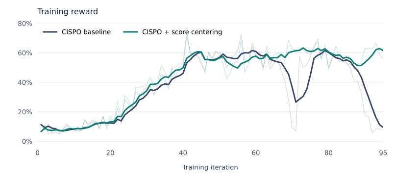
Score centering prevented collapse in this comparison. By iteration 140, held-out answer correctness was 61.1%, versus 0% for the baseline, measured over 200 held-out problems with four samples each.

Get started

pip install --upgrade 'river-client[custom-loss]>=0.17.1'

Define the objective, declare its inputs, and call prepare_loss to use in your training run.

The same custom losses are supported in our RL SDK via rl.CustomLoss that connects custom objectives to AsyncTrainer. See the custom-loss guide for supported operations, RL SDK integration and more examples.

References

1. Thinking Machines Lab. Custom Loss Functions.
2. TypeSafe AI. Introducing System One Models & Jev.
3. MiniMax. MiniMax-M1: Scaling Test-Time Compute Efficiently with Lightning Attention. 2025.
4. Martin Marek and Max Ryabinin. Score Centering Stabilizes Off-policy Reinforcement Learning. 2026.